
Editor's Note: Options are not suitable for all investors. Options involve risks, including substantial risk of loss and the possibility an investor may lose the entire amount invested in a short period of time. Please see the Characteristics and Risks of Standardized Options.
Table of Contents
- What Is the Binomial Option Pricing Model?
- Assumptions of the Binomial Option Pricing Model
- How Does the Binomial Model Work?
- Binomial Option Pricing Model Calculations
- Binomial Model Example
- Pros and Cons of the Binomial Model
- Binomial Option Pricing Model vs Black-Scholes Model
- Binomial Option Pricing Model vs Monte Carlo Model
- FAQ
The binomial option pricing model is a valuation tool that predicts the price of an asset for selected future points in time, then uses an iterative approach to work backwards to determine the present value of options on that underlying asset.
The binomial option pricing model has the benefit of being relatively easy to implement and provides visibility into the linkages between the underlying asset price and option prices as the expiration date approaches.
Key Points
• The binomial option pricing model estimates an option’s present value by forecasting possible asset prices at future points in time, then working backward through each period.
• The model assumes two possible outcomes at each node — an upward or downward move in the underlying asset’s price — which produces an iterative, path-dependent calculation.
• Unlike the Black-Scholes model, the binomial model accommodates American-style options where contracts exercise at any point before expiration.
• Key assumptions of the binomial option pricing model include no dividends, a constant risk-free rate, no transaction costs, and risk-neutral investor behavior throughout the pricing period.
• The binomial model’s relative simplicity and multi-period flexibility make it a practical alternative to more complex approaches, like the Monte Carlo simulation.
What Is the Binomial Option Pricing Model?
The binomial option pricing model is a widely used option pricing formula. There are multiple versions of the model, depending on what assumptions the trader wishes to make and what types of options are to be priced.
Fundamentally, the model involves a three-step process:
1. Generate the binomial price tree for the underlying asset.
2. Calculate the options values based on the asset prices for each final node.
3. Calculate the option value at each preceding node.
Recommended: How to Trade Options
Assumptions of the Binomial Option Pricing Model
The binomial option pricing model assumes two possible outcomes: an up or down change in the stock price. Although it’s simple in a one-period approach, the model can quickly turn complex over multiple time frames. However, constructing the pricing tree illustrates how an asset’s price changes from period to period.
Another advantage is that the binomial option pricing model can be used to value American, European, and Bermuda-style options (with modifications). There are adjustments needed to use the binomial model based on which options are being priced. For this discussion, the focus will be on American options only.
Other assumptions in the model discussed herein include that the underlying asset pays no dividends, the interest rate is unchanging, there are no transaction costs, there are no taxes, and that the risk-free rate does not change.
It also assumes investors are risk-neutral.
How Does the Binomial Model Work?
The binomial option tree is used for finding the current value of an option. This value is equal to the present value of the probability-weighted future payoffs.
Binomial Option Pricing Model Calculations
Let’s dive into calculations for calls and puts. In order to understand how these calculations are made it helps to know the basics of options trading strategies.
Call Options
A call option gives the holder the right, but not the obligation, to purchase a security at a specific price before expiration. A call option is in the money when the stock price is above the strike price. A binomial tree’s nodes will value an option at the maximum of zero or its calculated value.
Recommended: How Options Are Priced
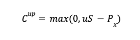
When the underlying asset moves up in price, the call option’s payoff (Cup) is the maximum of zero and the stock price (S) multiplied by the up factor (u) and reduced by the exercise price (Px).
When the underlying asset moves down in price, the call option’s payoff (Cdown) is the maximum of zero and the stock price (S) multiplied by the down factor (d) and reduced by the exercise price (Px).
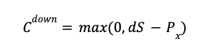
The binomial model calculates all possible payoffs, based on these calculations. The final outcomes are then discounted back to calculate the present value.
Put Options
Put options give the holder the right but not the obligation to sell a security at a specific price at a specific time. A put option is in the money when the stock price is less than the strike price.
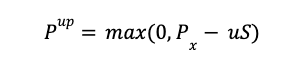
When the underlying asset moves up in price, the put option’s payoff (Pup) is the maximum between zero and the exercise price (Px) minus the stock price (S) multiplied by the up factor (u).
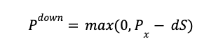
When the underlying asset moves down in price, the put option’s payoff (Pdown) is the maximum between zero and the exercise price (Px) minus the stock price (S) multiplied by the down factor (d).
Binomial Model Example
Assumptions
XYZ stock is currently trading at $100 and you wish to calculate the value of a call option with a $105 strike price that will expire in two weeks.
Assume that the stock may increase by 10% or decrease by 15% each week. The risk-free rate is currently 5%, and you will be looking for cash settlement rather than delivery of shares. Additionally, XYZ is not expected to pay dividends over the two-week holding period.
You want to view how the option price will move weekly up until expiration and calculate the option value today.
Generate the Binomial Tree
We construct the binomial tree for the prices of XYZ stock.
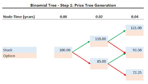
At the end of one week (1/52 of a year or 0.02 years) the stock will be priced at either $110 or $85.
After two weeks, (0.04 years) the price will increase to $121 if the price moves up twice in a row. The stock price will be $93.50 if the price moves up then down, or down then up. Finally, if the stock moves down twice in a row the stock will drop to $72.25.
Note that we can create a binomial tree for any time period size and include many more steps at the cost of greater complexity in the calculations.
Calculate Final Option Values
Having forecast the stock price two weeks into the future we can calculate the value of the $105 strike price call option at that time.
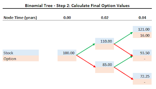
The call option will only have value if the stock moves up twice in a row. At that time the shares will be worth $121 and the option will be worth $16.
Stock price – Strike price = $121 – $105 = $16
Work Backward to Calculate Present Values
Before we can perform the present value calculations we need to determine the probability that the stock price, and the call option price, will move along the upward path in the binomial tree during each week.
Fortunately we have all the information we need to calculate the probability based on our initial assumptions. The probability for an up move is:
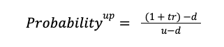
Where:
• t = the time period in years (1 week = 0.02 years)
• r = the risk-free rate (5%)
• u = up factor ($110 / $100 = 1.1)
• D = down factor ($85 / $100 = 0.85)
Substituting into the equation below:

Because there are only two paths at each node, the probability of a down move is:

Given the probabilities and the potential option values at the end of week two, we use the present value calculation to determine the option value for the end of week one.
We repeat this process until we arrive at the value of the call option today.
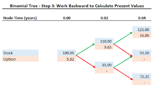
At each step we weigh the final values by their respective probabilities and discount by the risk-free rate using the following equation:


Finally, we arrive at the present value of the call option of $5.82.
Finally, user-friendly options trading is here.*
Trade options with SoFi Invest on an easy-to-use, intuitively designed online platform.
*Check out the OCC Options Disclosure Document.
Pros and Cons of the Binomial Model
thumb_up
Pros:
• Simple to calculate
• Can be used on American options
• Can be used over multiple periods
thumb_down
Cons:
• Difficult to predict future prices and probabilities
• Assumes conditions that are not seen in real-world markets
• Complexity grows as more periods are considered
Binomial Option Pricing Model vs Black-Scholes Model
The Black-Scholes model comes to a deterministic result based on the inputs. Its inputs are option variables such as the strike price, the current stock price, the time to expiration, the risk-free rate, and the volatility. While the binomial model is considered path dependent, the Black-Scholes model is path independent.
Widely used in practice and considered accurate, the Black-Scholes model makes assumptions that sometimes arrive at options prices that are different from those seen in the real world.
The Black-Scholes model is considered the standard when valuing European options since the model does not allow for options to be exercised early.
| Binomial Option Pricing Model | Black-Scholes Model |
|---|---|
| Probabilistic approach | Deterministic approach |
| Path dependent with two possible outcomes at each node | Usually accurate, but output prices sometimes deviate from those seen in the real world |
| Helpful for American options | Helpful for European options |
Binomial Option Pricing Model vs Monte Carlo Model
The Monte Carlo model runs thousands of computer simulations to arrive at a solution. Monte Carlo simulation often includes an array of possible paths — some that show higher ending prices and others that show lower prices.
The computer simulations are only as good as the assumptions used. Analysts can tailor the inputs. Often, historical data is used in Monte Carlo simulations which may lead to results that aren’t applicable.
| Binomial Option Pricing Model | Monte Carlo Model |
|---|---|
| An iterative approach that is path dependent | Based on computer simulations |
| Less computer-intensive | You can tailor the inputs and scenarios |
| Uses future assumptions, not historical data | Output only as good as the assumptions used |
The Takeaway
The binomial option pricing model is a valuation tool that predicts the price of an asset for selected future points in time then uses an iterative approach to work backwards to determine the present value of options on that underlying asset.
Due to its relative simplicity and speed, traders may prefer the binomial model to the Black-Scholes and Monte Carlo models.
SoFi’s options trading platform offers qualified investors the flexibility to pursue income generation, manage risk, and use advanced trading strategies. Investors may buy put and call options or sell covered calls and cash-secured puts to speculate on the price movements of stocks, all through a simple, intuitive interface.
With SoFi Invest® online options trading, there are no contract fees and no commissions. Plus, SoFi offers educational support — including in-app coaching resources, real-time pricing, and other tools to help you make informed decisions, based on your tolerance for risk.
Explore SoFi’s user-friendly options trading platform.
FAQ
Who developed the binomial model?
The binomial options pricing model was first suggested by William Sharpe in 1978, but the model’s development is associated with work done by John Cox, Stephen Ross, and Mark Rubinstein in 1979.
Are the Black-Scholes and binomial option pricing models the same?
No, these are two different models. The Black-Scholes model provides a numerical result based on inputs. The binomial options pricing model prices an asset based on a range of possible results. The binomial model is considered an iterative calculation since there is a range of possible outcomes to value options. The Black Scholes model uses fixed inputs to arrive at an option’s value.
How is the binomial option pricing model different from the Monte Carlo model?
The Monte Carlo model runs thousands of computer simulations to eventually arrive at an options price. The model first generates a random number based on a probability distribution. That number then uses additional option inputs like volatility and time to expiration to generate a stock price. The stock price at expiration is then used to calculate the value of the option.
The model runs this process thousands of times, each using different variables from the probability functions. To determine option pricing, the Monte Carlo model uses the average of all the calculated results.
Photo credit: iStock/David Petrus Ibars
INVESTMENTS ARE NOT FDIC INSURED • ARE NOT BANK GUARANTEED • MAY LOSE VALUE
Options involve substantial risk of loss and the possibility an investor may lose the entire amount invested. Before starting options trading, investors should be familiar with the Characteristics and Risks of Standardized Options . TTax implications with options should be considered. Consult your tax advisor to understand any impacts to your taxes.
Financial Tips & Strategies: The tips provided on this website are of a general nature and do not take into account your specific objectives, financial situation, and needs. You should always consider their appropriateness given your own circumstances.
Disclaimer: The projections or other information regarding the likelihood of various investment outcomes are hypothetical in nature, do not reflect actual investment results, and are not guarantees of future results.
Tax Information: This article provides general background information only and is not intended to serve as legal or tax advice or as a substitute for legal counsel. You should consult your own attorney and/or tax advisor if you have a question requiring legal or tax advice.
SOIN-Q425-030